Bioinformatics by hand: Neighbor-joining trees

Hi! I'm Amelia Harrision, Pokémon master, Bioinformatics trainer, and workshop developer @ UD. Contact me on LinkedIn!
Contents
Bioinformatics by hand
I’ve been teaching bioinformatics at the University of Delaware for roughly the last year now. I had never been in a bioinformatics class prior to teaching; my degrees are in ecology and marine science, so all of my bioinformatics knowledge came from research experience. It’s been really interesting to see bioinformatics taught in a formal setting. One thing I’ve noticed is the disconnect that can occur between students and instructors when students without programming experience are asked to perform “hands-on” exercises.
In an effort to de-mystify bioinformatics, instructors often have students manually perform a task that would normally be done computationally. While these exercises are valuable and often succeed in their goal, I have noticed that many students who are not used to being presented with code or equations tend to have difficulty implementing algorithms by hand, regardless of difficulty. This can cause students to shut down and question whether they are in the correct field, rather than empower them.
When this occurs, there seem to be two underlying issues: First, even at the collegiate level, many students are not confident in their ability to do math. This issue I will leave alone, as it cannot be solved in a single course or assignment at the graduate level. Second, the way that a computer would perform a procedure is not necessarily the same way a human would perform it. Sometimes, this can create a gap between students with little or no computing background and instructors who are highly familiar with algorithms.
In this post, I’ll walk you through the process of building neighbor-joining trees. Building phylogenetic trees by hand seems at first like a daunting task, but I promise it’s much easier than you think!
Neighbor-joining trees
Neighbor-joining (NJ) is one of many methods used for creating phylogenetic (evolutionary) and phenetic (trait-based similarity) trees. The method was first introduced in a 1987 paper and is still in use today.
Neighbor-joining uses a distance matrix to construct a tree by determining which leaves are “neighbors” (i.e., children of the same internal parent node) via an iterative clustering process. A neighbor joining tree aims to show the minimum amount of evolution needed to explain differences among objects, which makes it a minimum evolution method.
There has been some debate about the mathematical behavior of neighbor-joining trees. Originally, neighbor joining was thought to be most closely related to tree methods that use ordinary least squares to estimate branch lengths, but further investigation showed that they actually shared more properties with “balanced” minimum evolution methods. You don’t need to know anything about these different methods in order to perform neighbor joining, but if you would like to read more about them, there is an excellent explanation in this paper.
The type of tree produced depends on the input. If you provide a distance matrix based on evolutionary data (e.g., multiple sequence alignment), you will get a phylogenetic tree. If you input distances based on non-evolutionary data (e.g., phenotypic traits), then you will get a phenetic tree. Note that a NJ tree doesn’t have to contain only organisms. You can make NJ trees for anything you can represent/compare with a distance matrix.
NJ trees are simple to make and require only basic operations (addition, subtraction, division), but can seem daunting because of the number of steps required. Here, I will show you how to make two small neighbor-joining trees by hand (or, by spreadsheet).
Pros and cons of neighbor-joining trees
There are a lot of different ways to build phylogenetic and other trees, so how does neighbor-joining compare?
Advantages
- It’s simple and easy to understand.
- It’s fast and computationally inexpensive compared to other popular methods. Maximum-likelihood and Bayesian methods especially are much slower.
- It works. Neighbor-joining has been found to be topologically accurate and to sometimes out-perform more complicated methods like maximum-likelihood and Bayesian inference.
Disadvantages
- You lose data. When you squish down sequence alignment or other data into distances, you are performing data reduction. This isn’t necessarily a bad thing (ordination methods like PCA also do this), but you should keep it in mind.
- You only get one possible tree. Other methods such as maximum-likelihood and Bayesian inference return multiple different trees, i.e. evolutionary hypotheses, which can be useful for some analyses.
- Neighbor-joining can sometimes result in negative branch lengths. Note that this does not affect the topology of the tree, just branch lengths.
How to neighbor-join
To begin neighbor-joining, you need a distance matrix. A distance matrix is a square matrix containing pairwise distances between members of some group. It must be symmetric (e.g., the distance from A to B is the same as the distance from B to A) and the distance from an object to itself must be 0. The distance does not necessarily need to be metric, but in at least one instance a metric distance slightly outperformed a non-metric distance.
Once you have a matrix, you can begin neighbor-joining.
The neighbor-joining process consists of three steps:
- Initiation
- Iteration
- Termination
A quick note on the formulas (which can be found in the section below this one): You may notice a slight difference in the equations between this tutorial and another. Do not panic. These are only slight algebraic differences that do not affect the final answer, only the intermediate numbers.
Initiation
In the initiation step, we define a set of leaf nodes, T, and set L equal to the number of leaf nodes. These are the nodes at the “ends” of trees and therefore do not have any child nodes. You should have one leaf node for each item you want to compare. For example, if you are placing sequences on a tree, you will have one leaf node per sequence.
Iteration
The iteration step is where most of the action takes place. Virtually all of our calculations are made in this step, and, as the name implies, we will repeat these calculations over and over until some conclusion is reached.
First, we calculate the net divergence (r) of each leaf node. You can think of this as being essentially the distance from each leaf node to all of the others.
Next, we calculate the adjusted distance (D) between each pair of nodes, which is based on the pairwise distance in the starting matrix and the divergence of each node. The pair of nodes with the lowest adjusted distance are neighbors and share a parent node.
Next, we declare the parent node and calculate the distance from each of the neighbors to the shared parent. This is also the step where I like to add the siblings and parent to the tree.
At this point, our goal is to construct a new distance matrix. To do this, we remove the two nodes that we earlier determined to be neighbors from the distance matrix and replace them with the newly formed parent node. New pairwise distances (d) are calculated between the new parent node and other nodes in the matrix. Any other distances (i.e., pairwise comparisons present in the new matrix and the previous matrix) can simply be transferred to the new matrix.
Note: In the formulas and calculations below, adjusted distances use a capital D, whereas pairwise distance use a lowercase d. Try not to get them mixed up!
One thing to be aware of is that, after the first iteration, the neighbors are not restricted to being leaves, and may in fact be internal parent nodes.
Each iteration step ends with a new distance matrix that is one node smaller than the one in the previous step (e.g., (L-1) by (L-1) after the first iteration). Iteration continues until there are only two nodes remaining in the matrix.
Termination
The final step is termination.
The only task remaining is to join the two nodes that remain after iteration with a single edge to complete the tree!
Now that we’ve braved the written explanation, it’s time to look at some examples to make all of these steps clearer!
Formulas
These are the formulas for each of the calculations we will perform (you can find more formatted version in the excel file containing the examples).
Net divergence
Net divergence r for a node i with 3 other nodes (j, k, and l):
r(i) = [1/(L-2)] \* [d(ij) + d(ik) + d(il)]Adjusted distance
Adjusted distance D for two nodes i and j:
D(ij) = d(ij) - [r(i) + r(j)]Distance from child to parent
Distance from child i to parent k, d(ik), where j is the neighbor of i:
d(ik) = [d(ij) + r(i) + r(j)] / 2Distance from non-child to new node
Distance from other non-child node, m to new node d(mk):
d(mk) = [d(im) + d(jm) - d(ij)] / 2Example 1
There’s a good chance that even if you read the description of neighbor-joining above, you still don’t have a great idea of how to do it. That should become clearer with some examples.
Here is our starting matrix:
| A | B | C | D | |
|---|---|---|---|---|
| A | 0 | 4 | 5 | 10 |
| B | 4 | 0 | 7 | 12 |
| C | 5 | 7 | 0 | 9 |
| D | 10 | 12 | 9 | 0 |
Step 1: Initiation
All we do here is define a set of leaf nodes, T, and set L equal to the number of leaf nodes.
T = { A, B, C, D }

L = 4
Step 2: Iteration
Now for the real action. Remember, this will consist of multiple iterations.
Iteration 1
First, we calculate the net divergence r of each node:
r(A) = [1/(L-2)] * [d(AB) + d(AC) + d(AD)] = (1/2) * (4 + 5 + 10) = 9.5

r(B) = [1/(L-2)] * [d(AB) + d(BC) + d(BD)] = (1/2) * (4 + 7 + 12) = 11.5

r(C) = [1/(L-2)] * [d(AC) + d(BC) + d(CD)] = (1/2) * (5 + 7 + 9) = 10.5

r(D) = [1/(L-2)] * [d(AD) + d(BD) + d(CD)] = (1/2) * (10 + 12 + 9) = 15.5
Next, the adjusted distance D for each node pair:
D(AB) = d(AB) - [r(A) + r(B)] = 4 - (9.5 + 11.5) = -17

D(AC) = d(AC) - [r(A) + r(C)] = 5 - (9.5 + 10.5) = -15

D(AD) = d(AD) - [r(A) + r(D)] = 10 - (9.5 + 15.5) = -15

D(BC) = d(BC) - [r(B) + r(C)] = 7 - (11.5 + 10.5) = -15

D(BD) = d(BD) - [r(B) + r(D)] = 12 - (11.5 + 15.5) = -15

D(CD) = d(CD) - [r(C) + r(D)] = 9 - (10.5 + 15.5) = -17
The pair of nodes with the smallest adjusted distance are neighbors. In this case, we have a tie between the pairs AB and CD. We can only move forward with one pair, so we’ll pick AB. We now define a new node that connects these neighbors; we’ll call this new node Z.
We’re close now to constructing our first bit of the tree. To do that, we need to calculate the distance from each neighbor (child) node to the connecting (parent) node.
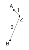
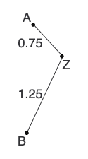
d(AZ) = [d(AB) + r(A) - r(B)]/2 = (4 + 9.5 - 11.5)/2 = 1

d(BZ) = [d(AB) + r(B) - r(A)]/2 = (4 + 11.5 - 9.5)/2 = 3
With this information, we can draw the first two branches on our tree:
Lastly, we need to reconstruct the distance matrix, replacing A and B with Z. Some distances can be transferred, but others (represented by question marks), need to be calculated:
| Z | C | D | |
|---|---|---|---|
| Z | 0 | ? | ? |
| C | ? | 0 | 9 |
| D | ? | 9 | 0 |
Here are the formulas for calculating d(ZC) and d(ZD).
d(ZC) = [d(AC) + d(BC) - d(AB)]/2 = (5 + 7 - 4)/2 = 4

d(ZD) = [d(AD) + d(BD) - d(AB)]/2 = (10 + 12 - 4)/2 = 9
With these calculations done, we can replace the question marks in our distance matrix:
| Z | C | D | |
|---|---|---|---|
| Z | 0 | 4 | 9 |
| C | 4 | 0 | 9 |
| D | 9 | 9 | 0 |
And we’re done…with the first iteration. Remember, the iteration step ends when there are only two nodes left in the matrix, and we have three. On to the next iteration!
Iteration 2
For this iteration, we use the latest version of the distance matrix, constructed at the end of the previous iteration and reset L (the number of nodes in the matrix).
L = 3Calculate the net divergence r of each node:
r(Z) = [1/(L-2)] * [d(ZC) + d(ZD)] = 1 * (4 + 9) = 13

r(C) = [1/(L-2)] * [d(ZC) + d(CD)] = 1 * (4 + 9) = 13

r(D) = [1/(L-2)] * [d(ZD) + d(CD)] = 1 * (9 + 9) = 18
Next, the adjusted distance D for each node pair:
D(ZC) = d(ZC) - [r(Z) + r(C)] = 4 - (13 + 13) = -22

D(ZD) = d(ZD) - [r(Z) + r(D)] = 9 - (13 + 18) = -22

D(CD) = d(CD) - [r(C) + r(D)] = 9 - (13 + 18) = -22
All of the pairs are tied for lowest adjusted distance, so we’ll select ZC because it’s first in the list and define a new node Y that connects the neighbors.
Calculate the distances from the new parent node to it’s children:
d(ZY) = [d(ZC) + r(Z) - r(C)]/2 = (4 + 13 - 13)/2 = 2

d(CY) = [d(ZC) + r(C) - r(Z)]/2 = (4 + 13 - 13)/2 = 2
Add the new branches to the tree:
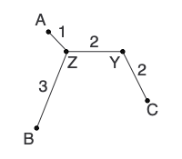
Calculate any other new distances and construct the new distance matrix:
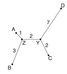
d(YD) = [d(ZD) + d(CD) - d(ZC)]/2 = (9 + 9 - 4)/2 = 7| Y | D | |
|---|---|---|
| Z | 0 | 7 |
| D | 7 | 0 |
Step 3: Termination
L now consists of only 2 nodes (Y and D), so we add the edge between them to finish the tree:
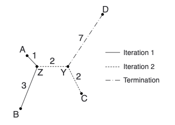
Summary
And with that, we’ve built our first neighbor-joining tree! Here is the tree coming together in each step:
On Distance Matrices
Now, you may have noticed that to build the tree in Example 1, we didn’t actually need all of those formulas. In iteration 1, for example, we can figure out the distance from A and B to their parent just by noticing that B is always 2 units further from other nodes than A. Therefore, d(BZ) must equal d(AZ) + 2. If their combined distance from Z is 4, then the only possible branch lengths are 1 and 3.
So, why did we go through the trouble of neighbor-joining? And when do we actually need neighbor-joining?
Additive matrices
The distance matrix that we used for example 1 is what’s called an additive matrix. Simply put, a matrix is additive if you are able to reproduce the starting matrix by adding together the branch lengths along the paths between nodes. To demonstrate this, let’s look back at example 1.
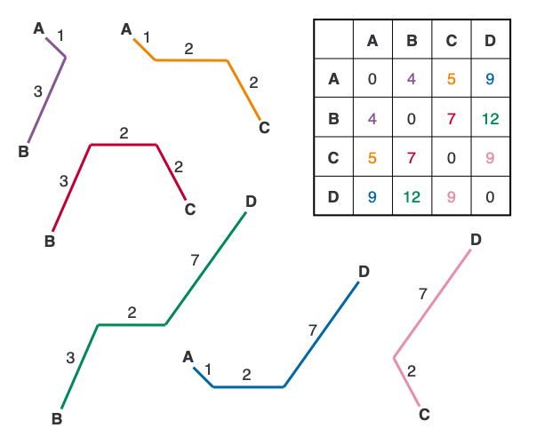
In the figure above, I’ve deconstructed the tree so that you can see the individual paths between each pair of leaf nodes. Notice that we can reconstruct the starting matrix exactly using only the distances on the tree, which is the main trait of an additive matrix (for a more technical and thorough look at additive matrices, see this presentation).
I like to use an additive matrix as the first neighbor-joining example because, 1) it gives me an excuse to discuss additive matrices, and 2) it’s very easy to check your work. If you are unable to reconstruct the starting matrix in example 1 using the tree, you know you have a problem in your calculations, which is harder to catch with non-additive matrices.
Alright, so if we don’t need neighbor-joining for additive distance matrices, then when do we need it? Neighbor-joining is said to work best for near-additive matrices, i.e. matrices for which the tree almost reconstructs the starting matrix, though they have been reported to be topologically accurate even when this is not the case. And I should note here that the vast majority of distance matrices based on biological data are not additive or even nearly additive.
Without further ado, here is another example using a nearly-additive matrix.
Example 2
Here is our starting matrix:
| A | B | C | D | |
|---|---|---|---|---|
| A | 0 | 2 | 2 | 2 |
| B | 2 | 0 | 3 | 2 |
| C | 2 | 3 | 0 | 2 |
| D | 2 | 2 | 2 | 0 |
Step 1: Initiation
Again, we define T and L. They are the same as example 1.
T = { A, B, C, D }

L = 4
Step 2: Iteration
Iteration 1
First, we calculate the net divergence r of each node:
r(A) = [1/(L-2)] * [d(AB) + d(AC) + d(AD)] = (1/2) * (2 + 2 + 2) = 3

r(B) = [1/(L-2)] * [d(AB) + d(BC) + d(BD)] = (1/2) * (2 + 3 + 2) = 3.5

r(C) = [1/(L-2)] * [d(AC) + d(BC) + d(CD)] = (1/2) * (2 + 3 + 2) = 3.5

r(D) = [1/(L-2)] * [d(AD) + d(BD) + d(CD)] = (1/2) * (2 + 2 + 2) = 3
Next, the adjusted distance D for each node pair:
D(AB) = d(AB) - [r(A) + r(B)] = 2 - (3 + 3.5) = -4.5

D(AC) = d(AC) - [r(A) + r(C)] = 2 - (3 + 3.5) = -4.5

D(AD) = d(AD) - [r(A) + r(D)] = 2 - (3 + 3) = -4

D(BC) = d(BC) - [r(B) + r(C)] = 3 - (3.5 + 3.5) = -4

D(BD) = d(BD) - [r(B) + r(D)] = 2 - (3.5 + 3 = -4.5

D(CD) = d(CD) - [r(C) + r(D)] = 2 - (3.5 + 3) = -4.5
A lot of ties here. Again, we’ll pick the tied pair that is closest to the top of the list, AB, and assign them a parent node, Z.
Now, calculate the distance from each neighbor (child) node to the connecting (parent) node.
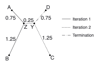
d(AZ) = [d(AB) + r(A) - r(B)]/2 = (2 + 3 - 3.5)/2 = 0.75

d(BZ) = [d(AB) + r(B) - r(A)]/2 = (2 + 3.5 - 3)/2 = 1.25
And draw the first two branches on our tree:
Lastly, we calculate new distances and reconstruct the distance matrix:
d(ZC) = [d(AC) + d(BC) - d(AB)]/2 = (2 + 3 - 2)/2 = 1.5

d(ZD) = [d(AD) + d(BD) - d(AB)]/2 = (2 + 2 - 2)/2 = 1| Z | C | D | |
|---|---|---|---|
| Z | 0 | 1.5 | 1 |
| C | 1.5 | 0 | 2 |
| D | 1 | 2 | 0 |
On to the next iteration!
Iteration 2
For this iteration, we use the latest version of the distance matrix, constructed at the end of the previous iteration and reset L.
L = 3Calculate the net divergence r of each node:
r(Z) = [1/(L-2)] * [d(ZC) + d(ZD)] = 1 * (1.5 + 1) = 2.5

r(C) = [1/(L-2)] * [d(ZC) + d(CD)] = 1 * (1.5 + 2) = 3.5

r(D) = [1/(L-2)] * [d(ZD) + d(CD)] = 1 * (1 + 2) = 3
Next, the adjusted distance D for each node pair:
D(ZC) = d(ZC) - [r(Z) + r(C)] = 1.5 - (2.5 + 3.5) = -4.5

D(ZD) = d(ZD) - [r(Z) + r(D)] = 1 - (2.5 + 3) = -4.5

D(CD) = d(CD) - [r(C) + r(D)] = 2 - (3.5 + 3) = -4.5
All of the pairs are tied for lowest adjusted distance, so we’ll select ZC because it’s first in the list and define a new node Y that connects the neighbors.
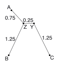
Calculate the distances from the new parent node to it’s children:
d(ZY) = [d(ZC) + r(Z) - r(C)]/2 = (1.5 + 2.5 - 3.5)/2 = 0.25

d(CY) = [d(ZC) + r(C) - r(Z)]/2 = (1.5 + 3.5 - 2.5)/2 = 1.25
Add the new branches to the tree:
Calculate any other new distances and construct the new distance matrix:
d(YD) = [d(ZD) + d(CD) - d(ZC)]/2 = (1 + 2 - 1.5)/2 = 0.75| Y | D | |
|---|---|---|
| Z | 0 | 0.75 |
| D | 0.75 | 0 |
Step 3: Termination
L now consists of only 2 nodes (Y and D), so we add the edge between them to finish the tree:
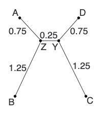
Summary
Here is our second tree in completion:
Lastly, let’s make a distance matrix using the tree to provide the distances. Notice that these distances are just a little bit off from the starting matrix. Hence, “near-additive”.
| A | B | C | D | |
|---|---|---|---|---|
| A | 0 | 2 | 2.25 | 1.75 |
| B | 2 | 0 | 2.75 | 2.25 |
| C | 2.25 | 2.75 | 0 | 2 |
| D | 1.75 | 2.25 | 2 | 0 |
Wrapping up
Having reached the end of this lesson, you should have learned how to construct neighbor-joining trees by hand from additive and nearly additive matrices. If you want to take a closer look at the examples (and access one additional example), you can check out this excel file.
If you enjoyed this post, consider sharing it on Twitter or LinkedIn and subscribing to the RSS feed! If you have questions or comments, you can find me on LinkedIn or send me an email directly.
← Go back